Ch. 1: Introduction
INTRODUCTION
Making good maps can be challenging, time consuming, and expensive, but recently, a new set of cheap and free mapping tools has enabled almost anyone with a computer to easily make a map—but good maps are not usually the result. They have the computer and software, but the new mapmakers lack the mapping concepts, principles, and methodologies. Their maps are often improperly designed and do not communicate easily nor effectively.
This e-text wants to change that by helping you create, analyze, and produce maps that communicate more effectively. By the use of symbols, colors, shades, and words, maps help us communicate with more impact; they make what we want to say attractive, compelling, convincing, and clear. This e-text focuses primarily on a technology called Geographic Information Systems (GIS), but most of the chapter’s concepts are applicable to other geotechnologies including remote sensing, global positioning systems (GPS), Internet mapping, and virtual globes.
DEFINITIONS OF GEOGRAPHIC INFORMATION SYSTEMS (GIS)
Let’s define GIS first.
Definition #1
Over the past 20 to 30 years, many authors (Dept of the Environment, 1987; Rhind, 1988; Parker, 1988; and Bolstad, 2002) have defined GIS, and most of their definitions are similar to one another. The definitions generally refer to a system of computer hardware, software, and people that support the capture, management, analysis, and display of spatial data.
It is a decent definition, but to understand GIS better, you should break it down into its four main subsystems the way Marble and Peuquet (1983) did in perhaps the first widely used GIS textbook. GIS have:
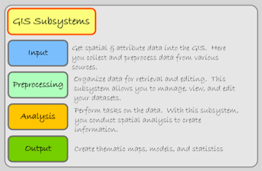
Figure 1.1: The four GIS subsystems.
Much of this e-text is divided into chapters that mirror these four GIS subsystems. Chapter 2 looks at data and the data input system. Chapters 3 and 4 focus on the graphic and database portions of GIS software. These two chapters finish by covering various “housecleaning” processes (preprocessing functions) that manipulate the data files to make them ready for analysis. Chapter 5 looks at how to analyze the datasets. Output is covered in Chapter 6.
Definition #2
An even shorter definition equates GIS to a “spatial database”, but you must focus on both of those words carefully. To do this, think of a computer screen displaying a simple parcel map.
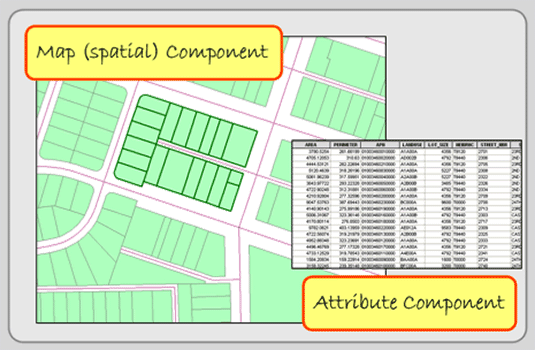
Figure 1.2: The two parts of a GIS.
Each parcel is a separate feature on the map, but they are more than just features on the screen, the computer stores many database characteristics about the feature like the parcel’s identification number and its owner’s name. In other words, there are two parts to a GIS: a map (or spatial) component and an attribute (or database) component. By making this link between the map and the stored attributes, GIS becomes a powerful tool for addressing and analyzing geographic data and environmental issues. This is its appeal. GIS programs are capable of handling large and diverse geographic datasets, and we increasingly rely upon them for analyzing and making decisions.
The two definitions above emphasize GIS as a computer system; a simple definition for a computer system differs only in that GIS handles spatial data. Although the second definition gets closer, both definitions, do not give adequate weight to the geographic component of GIS.
Definition #3
It is no accident that GIS begins with G. A good understanding of GIS begins with geography and specifically with a geographic perspective, which is a way of organizing and thinking about portions of the Earth spatially. Again, look at the map above. You know that it and many other maps depict the locations of people and things (like roads, important buildings, parks, etc.). You also know that there are connections or relationships between the people and things drawn on the map. These relationships help explain the spatial patterns you see on the map. The process of finding, showing, explaining, and even predicting geographic patterns is at the heart of both geography and GIS.
In this context, GIS can be defined as a tool of exploration that helps us explore geographic (or spatial) patterns. At a minimum, it aids us in describing these patterns, but GIS can go beyond simply description to help us investigate and understand why these patterns (sometimes called distributions) exist, the impacts these patterns have on our life and land, and to discover potential future geographic patterns.
You can address five types of geographic questions with GIS and other geotechnologies (ESRI, 1992, pp):
- What is at…? This basic question looks at what is at a particular location. An example might include, what is at the corner of Main Street and 12th Avenue?
- Where is it? This question could simply inquire as to the location of something specific (like the nearest market or bookstore), or it can be a more challenging question that explores what locations meet a specific condition. For example, a city might identify all of the parcels that are larger than 5 acres, vacant, zoned commercial, and within ½ mile of a freeway on-ramp.
- What has changed since? Over a portion of the Earth’s surface, how have conditions changed over time? An example is a county that identifies wetland areas that have decreased in size over the past 10 years.
- What spatial patterns exist? This question describes and compares spatial patterns at different locations. It attempts to find spatial patterns—perhaps the concentration of phenomena. The process of finding, showing, and explaining geographic patterns is frequently termed spatial analysis. Stewart Fotheringham defines spatial analysis as manipulating spatial data to extract additional meaning. In a GIS context, spatial analysis asks two questions:a. What is the relationship between two or more datasets that occupy the same location? For instance, you might see a direct relationship between a region’s varying elevation and the amount of rainfall that falls across it.
b. What geographic variations exist over space? All geographic phenomena vary in their intensity over space. Consider fertility rates across the United States. Some areas are high and others low. To answer this question fully, you need to describe and explain these patterns. - What if…? “What if?” questions involve scenarios that differ when you change the model’s parameters. An example includes looking at what happens to an area’s population when a freeway is built through the area under different constraints.
These questions examine relationships among various geographic phenomena, and you use GIS and other geotechnologies to explore and help you answer these questions. As the geographer Ron Abler states, “GIS technology is to geographical analysis what the microscope, the telescope, and computers have been to other sciences…” (1988, 40). No other technology looks so closely at the spatial relationship of phenomena, and it aids geographers and others that use spatial data to describe, analyze, and predict spatial relationships and patterns. As the geographer Michael DeMers states, “We can now see deeper and farther than we could before, allowing us to map more of what is present on the landscape and to ask questions that could not have been imagined” (2003, 3).
MANUAL GIS AND COMPUTER-BASED GIS
Abler’s and DeMers’ quotes may give you the impression that GIS is a new concept. Although the term GIS has been around for more than 30 years, the concepts surrounding GIS are old, and even the practice of doing GIS began before computers. The difference today is that GIS is computerized, but there is nothing a computer can do that cannot be done, at least theoretically, by hand if you had enough time, money, and energy. Computers process numbers and mathematical equations far quicker and more accurately than people can by hand or with the use of a calculator. Yet, before the concepts behind GIS were transferred to computers, people were doing manual GIS. They just combined spatial and attribute data on various types of media including hard-copy maps, hard-copy overlays (acetate or vellum), aerial photographs, written reports, field notebooks, and—of course—their eyes and minds.
With manual GIS, a large base map was often placed on a tabletop, and a series of transparent overlay maps, drawn at the same scale, were placed on top of the base map. One would then look for relationships among the base map and the features on the transparent overlays. Frequently, spatial data were copied from one map (or aerial photograph) to another. This took time, and because of it, many great ideas about the relationships of the Earth’s features (both physical and human) were not analyzed. These ideas were constrained by the amount of time it took to do the analysis. Still, some impressive manual GIS projects did occur.
The much-repeated example of Dr. John Snow’s Cholera map is a great example of manual GIS. In the 1840s, a cholera outbreak killed several hundred residents in London’s Soho section. Snow, a physician, located the address of each fatality on a hand-drawn base map and soon a cluster of cases was visible (Figure 1.3).
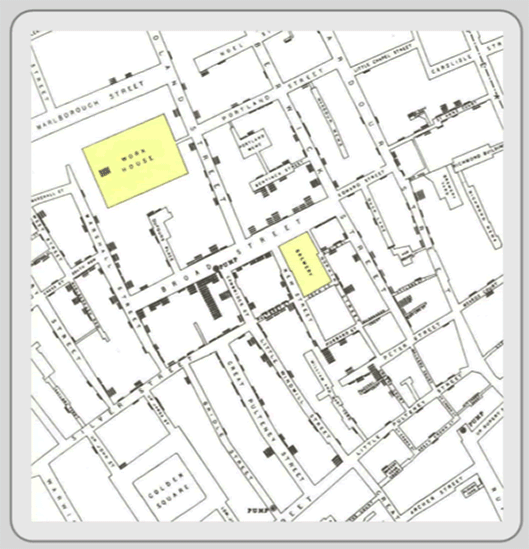
Figure 1.3: Dr. John Snow's Cholera Map of London's Soho.
Then on the base map, over the streets and fatalities, he drew the locations of water wells. Familiar with the idea of distance decay, he knew that people might go a far distance to purchase a product that was cheaper, but they would go to the nearest well because water was free and heavy to carry. Snow could see that the fatalities clustered largely among those who lived near the Broad Street water well. He and his students took the handle off the water pump, and new cholera cases dropped rapidly. By disabling the pump, Snow demonstrated the spatial relationship between cholera fatalities and the Broad Street water well, and, more importantly, he established the relationship between cholera and drinking water.
Even with the advent of computers, it took decades for GIS applications to get to where they are today. The largest and most powerful computers were mainframes that were available to some academics and government officials, but not to many researchers. In the 1980s, most GIS applications ran on workstation computers tied to mainframe computers because the early microcomputers (IBM, Apple, etc.) did not have enough memory, storage capacity, or processing ability. Today’s personal computers, however, are fast, capable of storing and processing large datasets, and can process multiple tasks simultaneously. This enables many academics, government agencies (from local to federal), organizations, and small and large businesses to use GIS. Computer-based GIS has its advantages, but requires educated users.
GIS EDUCATION AND TRAINING
GIS, virtual globes, GPS, and remote sensing are revolutionizing and revitalizing the discipline of geography. This has greatly improved the outlook for geography students and others who use spatial data in securing jobs. Along with nanotechnology and biotechnology, the U.S. Department of Labor identified geotechnology as one of the three most important emerging and evolving fields of study (Gewin, 2004).
Despite the good news, students often run high on anxiety when it comes to securing future employment, and they often ask for advice on what they should study to secure a GIS position. They ask about software, course selection, whether they should get a certificate, and even what should be their major or specialization. GIS professionals, administrators, and academics all have their own ideas and biases, but it usually comes down to this question: What is more useful, GIS training or GIS education? Students can usually answer this question if they can answer another related question: Do you want to apply GIS or focus on the technology itself?
GIS Education
If you want a position using GIS, you need to obtain conceptually both a geographic perspective and an idea of what one can do with a GIS. Both of these are conceptual topics that primarily stay away from the practical details of any particular GIS program. The focus is on applying GIS to answer real-world or discipline specific questions. It involves knowing about your data sources, the real-world processes of your discipline, and how one can use GIS to answer specific questions. GIS software training is a by-product, not the focus.
Specifically, a GIS education should provide students with:
- A geographic perspective. This is the process of finding, showing, explaining, and predicting geographic patterns (discussed briefly under the third GIS definition above).
- GIS concepts and cartographic principles. GIS concepts like buffering and overlay have their origin outside of GIS, but a number of procedures like these are closely tied to the technology. After becoming familiar with these processes, you need to determine which specific GIS processes are needed—and the order of these processes—to complete your projects. As Adena Schutzberg suggests, your objective is to “…get your head around how GIS ‘thinks” (Schutzberg, 2003).
GIS Training
Who would argue that training is not important? No doubt, businesses and agencies benefit when new hires already have the training to run their specific software programs. That said, it is easier to train someone in the use of a specific program if they understand the underlying concepts.
The problem with most GIS training is that the trainees are learning how to perform a specific set of routines. They are not primarily learning the spatial concepts relating to those routines although they may be secondarily obtained with work experience. Yes, training is important, but you will not “get your head around how GIS thinks” with training alone. Many of the jobs associated with training alone are data entry jobs that many might find tedious over time and frequently one’s advancement is limited. To avoid this, but stick to the training route, one can develop extensive database and programming skills. With these skills, you can usually rise up to better paying positions.
GIS Experience
Perhaps the best piece of advice I could give is that both education and training are important, but so is on-the-job experience. For those just starting out, GIS experience comes in a couple forms: internships and research assistantships.
An internship is a valuable way to obtain on-the-job experience. A good internship allows you to be part of the agency or organization’s day-to-day activities. They are usually commonly available, especially with government agencies.
To find these opportunities, talk with your academic advisor, go to your campus’s career services office, network at GIS seminars and meetings, or go directly to government agencies, organizations, and local companies that interest you. If you go directly to agencies, organizations, and businesses, you should provide the name of a faculty member as a reference, an updated resume, and you may want to volunteer your services.
Be sure that you have the appropriate skills for the internship and that you stick with the internship for a specified period. If you leave it abruptly, it hurts the chances of future students because many businesses and agencies have a tenuous relationship with internships in general, and they might decide that interns are too much trouble. Think of internships as necessary work experience.
Internships are important because you are more employable after this experience, it provides you with a list of contacts for future job opportunities, and it gives you a sense of the type of job you might want after college. Additionally, you may be offered a position at the agency where you interned.
Research assistantships are student positions where you assist a faculty member with the faculty member’s research. Some of these assistantships may involve GIS or other geotechnologies. Assistantships are available in many university academic departments, especially those that have graduate programs. Interested students should contact the department directly. Usually the assistantships are supported by external grant funding, so they are temporary positions but valuable experiences.
CONCEPTS
MAPS AS A MODEL OF REALITY
The real world is too complex and unmanageable for direct analysis and understanding because of its countless variability and diversity. It would be an impossible task to describe and locate each city, building, tree, blade of grass, and grain of sand. How do we reduce the complexity of the Earth and its inhabitants, so we can portray them in a GIS database and on a map? We do it by selecting the most relevant features (ignoring those we do not think are necessary for our specific research or project) and then generalizing the features we have selected. Chapter 6, as well as later portions of this chapter, covers the selection and generalization process in more detail. For now, let’s focus on features.
FEATURES
As described in Definition #2 (and Figure 1.2), conceptually, there are two parts of a GIS: a spatial or map component and an attribute or database component. Features have these two components as well. They are represented spatially on the map and their attributes, describing the features, are found in a data file. These two parts are linked. In other words, each map feature is linked to a record in a data file that describes the feature. If you delete the feature’s attributes in the data file, the feature disappears on the map. Conversely, if you delete the feature from the map, its attributes will disappear too.
Features are individual objects and events that are located (present, past or future) in space. In Figure 1.2, a single parcel is an example of a feature. Within the GIS industry, features have many synonyms including objects, events, activities, forms, observations, entities, and facilities. Combined with other features of the same type (like all of the parcels in Figure 1.2), they are arranged in data files often called layers, coverages, or themes. In this text, we use the terms feature and layer.
In Figure 1.4 below, three features—parcels, buildings, and street centerlines—of a typical city block are visible. Every feature has a spatial location and a set of attributes. Its spatial location describes not only its location but its extent. While “location” may be simple to grasp, it is difficult to locate features accurately and precisely. Accuracy and precision are examined in Chapter 2, but, in brief, precision deals with the exactness of the measurement. For example, some input devices, like GPS, have a certain error. They may be precise within a certain accuracy range if used correctly. Accuracy is the degree of correspondence between the data and the real world.
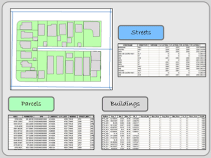
Figure 1.4: Each feature in the layers above has a spatial location and attribute data, which describes the individual feature.
Besides location, each feature usually has a set of descriptive attributes, which characterize the individual feature. Each attribute takes the form of numbers or text (characters), and these values can be qualitative (i.e. low, medium, or high income) or quantitative (actual measurements). Sometimes, features may also have a temporal dimension; a period in which the feature’s spatial or attribute data may change.
As an example of a feature, think of a streetlight. Now imagine a map with the locations of all the streetlights in your neighborhood. In Figure 1.5, streetlights most are depicted as small circles. Now think of all of the different characteristics that you could collect relating to each streetlight. It could be a long list. Streetlight attributes could include height, material, basement material, presence of a light globe, globe material, color of pole, style, wattage and lumens of bulb, bulb type, bulb color, date of installation, maintenance report, and many others.
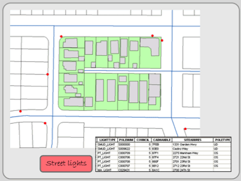
Figure 1.5: Location of street lights, represented with a red circle, and their attributes.
The necessary streetlight attributes depends on how you intend to use them. For example, if you are solely interested in knowing the location of streetlights for personal safety reasons, you need to know location, pole heights, and bulb strength. On the other hand, if you are interested in historic preservation, you are concerned with the streetlight’s location, style, and color.
Now continue thinking about feature attributes, by imagining the trees planted around your campus or office. What attributes would a gardener want versus a botanist? There would be differences because they have different needs. You determine your study’s features and the attributes that define the features.
POINTS, LINES AND POLYGONS
Now think of the feature’s shape on a map. Single or multiple paired coordinates (x, y) locate individual features in space and define their unique shape. The x and y values of each coordinate pair are associated with real world coordinate systems, which are discussed in Chapter 3. For now, let’s focus on the shape of features, which take the generalized form of points, lines, and polygons (see Figure 1.6).
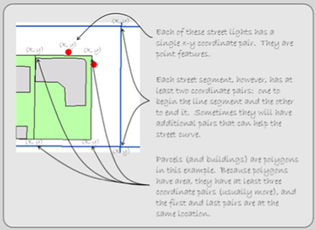
Figure 1.6: Each feature has a spatial position.
Points
Points are zero dimensional features (meaning that they possess only one x, y coordinate set) whose location is depicted by a small symbol. What you represent as a point depends on your study. Examples include streetlights, individual trees, wells, car accidents, crimes, telephone polls, earthquake epicenters, and even, depending on scale, buildings and cities.
Lines
Lines are formed from a sequence of at least two paired coordinates. The first pair starts the line and the last ends it. Two coordinate pairs form a straight line. Additional paired coordinates can form vertices between the starting and ending points that allow the line to bend and curve. Having length (which can be measured) but no width, a line feature is one-dimensional. Again, what is represented as a line depends on your study, but street centerlines, utility lines, canals, railroad tracks, rivers, flight paths, and elevation contour lines usually form lines.
Polygons
Polygons are features that have boundaries. Formed by a sequence of paired coordinates, polygons differ from lines in that the starting point is also its ending point. This provides polygons with both length and width, so these two-dimensional features can calculate the area contained within the feature. What is represented as a polygon differs from study to study, but examples include lakes, forest stands, buildings, counties, countries, states, and census districts.
TOPOLOGY
One of the most important concepts associated with GIS and other geotechnologies is topology. As features are added to a GIS, they form spatial relationships—called topology—with each other (both with features within the same layer and with features in different layers). You might find topology a confusing term partly because it has both spatial and mathematical properties. For our purposes, you can define it as the spatial relationships among features. It deals with where features are in relation to one another and how they are related to one another. These relationships take the form of simple distance calculations from one feature to another, but also include the more complicated issues of adjacency and connectivity.

Figure 1.7: Fire hydrants are located along streets (so fire trucks can connect) and adjacent to structures that can burn.
- Distances between features. The geographer Waldo Tobler created what some call the “first law of geography”, which states, “Everything is related to everything else, but near things are more related than distant things.” (1970, 236). This type of topology looks at the spatial relationships of where features are located. Consider the spatial locations of streets, bike lanes, sidewalks, and streetlights. They are positioned to work together. This is a type of topology; a relationship exists. Notice the relationship between the fire hydrant, building, and street in Figure 1.7.
- Adjacency. Adjacency focuses on a single type of feature (like streets or buildings) and whether parts of two or more individual features are shared (or contained). Think of an individual street segment, and how it is most likely physically connected to at least one additional street segment at one or both of its ends. These adjacent street segments are in turn connected to additional segments, which in turn are connected to streets, forming a network. When a single point or line (like a boundary between two parcels) is shared by at least two features, the spatial data file stores only a single point or a single line to prevent duplication that could lead to errors. This topological relationship describes how features are related.
- Connectivity. Also focusing on how features are related, connectivity specifies the way features are linked in a network. Even though a couple street segments may be physically connected in space, that does not mean that traffic can go in both directions. These are topological relationships that you can specify. Differing from adjacency, connectivity can include multiple feature types. For instance, you can determine the flow of water through connected pipe and valve features.
DATA MODEL
Current GIS programs represent points, lines, and polygons differently. There are two fundamental models: raster and vector. Each model has its advantages and disadvantages, and neither is superior to the other in every situation. One data model may fit certain types of data and applications better than the other.
Raster
A matrix of rows and columns, the raster data model covers sections of the Earth’s surface and represents features with cells or pixels. Pixels are the building blocks of the raster data model, and they are usually uniformly square and of consistent size within each layer. Each pixel represents a precise chunk of the Earth’s surface; the geographic position of any cell can be determined. A specific attribute value, representing the condition of that specific portion of the Earth’s surface (see figure 1.8), is associated with the pixel. If you need more than one attribute to describe the area contained within the pixel (and most likely you will), you need a second layer. The second raster layer gives you a second attribute. A third gives you a third attribute, and so on.
Individual cells and groups of cells represent the features of the real world (Figure 1.8). A point feature usually fills one cell while lines and polygons are constructed as a string or contiguous group of cells. Raster layers fill space; they describe what occurs everywhere in the study area. There are no blank spaces across the layer. “Empty” areas simply get a “0” value, but every pixel gets a value.
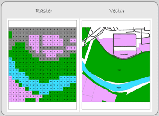
Figure 1.8: The raster and vector data models. Each stores features in a different way.
Conceptually, the raster model is simple. You take a portion of the Earth’s surface, divide it into cells, and give each cell an attribute that represents that area. In the figure above, you might give each cell either a D (developed), P (park), or W (water). For those cells with both park and water, you can give these cells either another code PW (for park and water) or make a judgment as to what covers the majority of the cell. Another way to code these cells is with the percentage of the cell that is water. If 40 percent of the cell is covered by water, the cell gets a value of 40.
Vector
The vector data model uses discrete point and line segments to identify the locations of the Earth’s features. Vector objects usually do not fill space like raster layers do; they depict where features occur and the space around those features is empty. Notice that there are white spaces in the vector model of Figure 1.8. No white spaces exist in the raster model; it covers the entire area.
Vector features are located with x, y coordinates. As described above, points are easy; they have one node (sometimes called a vertex). A node is a location in space that helps define the shape of point, line, and polygon features. As mentioned above, points have one coordinate pair that locates the feature in space. Lines have at least two nodes (their end points). Polygons have a minimum of three nodes to form an area. Lines and polygons usually have many more nodes that help define the course of the line or the polygon’s area.
Contrasting with raster systems that record one attribute per layer, the vector data model can handle many attributes for each feature type. Different software programs have varying ways of organizing vector digital files, but usually they have at least two files: one that stores spatial data and another that stores attributes.
The link between the spatial and attribute data files is made with a unique identifier. Each feature on the map and its corresponding attributes has a unique identifier that links the map feature to its database attributes. A type of unique identifier, a “key”, which links attribute files, is discussed in Chapter 3.
Raster versus Vector.
Which is better? Although GIS users have their own personal favorite data model, the question of which is “better” is an incomplete question. There are advantages and disadvantages to both data models, so a better question is which is better for particular applications or datasets. Some in the GIS industry use the slogan “Raster is faster, but vector is corrector.” While this is a good starting point, it conceals the details. Yes, your computer can process raster data quicker, but today computer processors are so fast the difference may be negligible. Yes, vector output looks more accurate, but you can increase pixel resolution to something resembling vector resolution (this, however, greatly increases the database size). The following are some of the advantages and disadvantages of the data models:
Raster advantages:
- Easy to understand. Conceptually, the raster data model is easy to understand. It arranges data into columns and rows. Each pixel represents a piece of territory.
- Processing speed. Raster’s simple data structure and its uncomplicated math produce quick results. For example, to calculate a polygon’s area, the computer takes the area contained within a single cell (which remains consistent throughout the layer) and multiples it by the number of cells making up the polygon. Likewise, the speed of many analysis processes, like overlay and buffering, are faster than vector systems that must use geometric equations.
- Data form. Remote sensing imagery is easily handled by raster-based systems because the imagery is provided in a raster format.
- Some analysis functions (surface analysis and neighborhood functions) are only feasible in raster systems. In addition, many new analysis functions appear in raster systems before migrating to vector systems because the math is simpler.
Raster disadvantages:
- Appearance. Cells “seem” to sacrifice too much detail (Figure 1.9). This disadvantage is largely aesthetic and can be remedied by increasing the layer’s resolution.
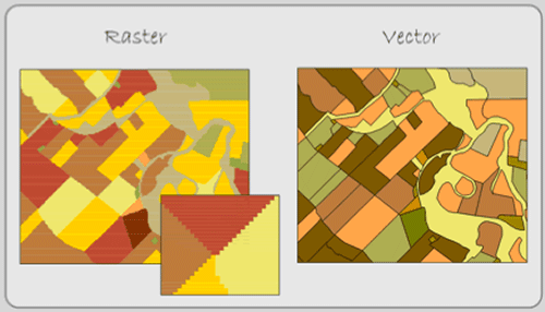
Figure 1.9: Comparison of raster and vector data models. Raster layers often appear pixilated and thus less accurate.
- Accuracy. Sometimes accuracy is a problem due to the pixel resolution. Imagine if you had a raster layer with a 30 by 30 meter resolution, and you wanted to locate traffic stop signs in that layer. The entire 30 by 30 meter pixel would represent the single stop sign. If you converted this raster layer to vector, it might place the stop sign at what was the pixel’s center. Sometimes problems of accuracy (and appearance) can be resolved by selecting a smaller pixel resolution, but this has database consequences.
- Large database. As just described, accuracy and appearance can be enhanced by reducing pixel size (the area of the Earth’s surface covered by each cell), but this increases your layer’s file size. By making the resolution 50 percent better (say from 30 to 15 meters), your layer grows four times. Improve the resolution again by halving the pixel size (to 7.5 meters) and your layer will again increase by four times (16 times larger than the original 30-meter layer). The layer quadruples because the resolution increases in both the x and y direction.
Vector advantages:
- Intuitive. In our minds, we picture features discreetly rather than made up of contiguous square cells.
- Resolution. If the locations of features are precise and accurate, you can maintain that spatial accuracy. The features will not float somewhere within a cell.
- Topology. Although the raster data model preserves where features are located in relation to one another, they do not represent how they are related to one another. This complex form of topology can be constructed in most vector systems, so you can track the connections in a municipal water network between pipe and valve features and thus track the direction and flow of water.
- Storage. Vector points, lines, and simple polygons use little disk space in comparison to raster systems. This was once a major consideration when hard-disk storage was limited and expensive.
Vector disadvantages:
- Geometry is complex. The geometrical algorithms needed for polygon overlay and the calculation of distances, depending on the projection/coordinate system used, require experienced programmers. This is not usually a problem for most GIS users since most functions are directly coded in the software.
- Slow response times. The vector data model can be slow to process complex datasets especially on low-end computers.
- Less innovation. Since the math is more complex, new analysis functions may not surface on vector systems for a couple of years after they have debuted on raster system.
